By Dr. Sam L. Savage
Why Everything is Behind Schedule, Beyond Budget & Below Projection
My dad was a mathematical statistician, and I remember a particular conversation with him about Jensen’s Inequality from about 60 years ago when I was a math major in college. I was about to take my first class in probability and statistics, and he was merely pointing out an important concept to keep in mind. That is:
The average value of a nonlinear function with uncertain inputs is NOT the value of the function given its average inputs.
It is notable that:
1. He brought this up out of the blue.
2. He did not mention any other concepts to keep in mind.
3. I don’t even recall the discussion of Jensen’s Inequality from my classes.
4. And neither does anyone else, apparently, because when I ask mathematicians or statisticians what it is, most have heard of it, but can’t tell me what it means.
5. It means that everything is Behind Schedule, Beyond Budget, and Below Projection!
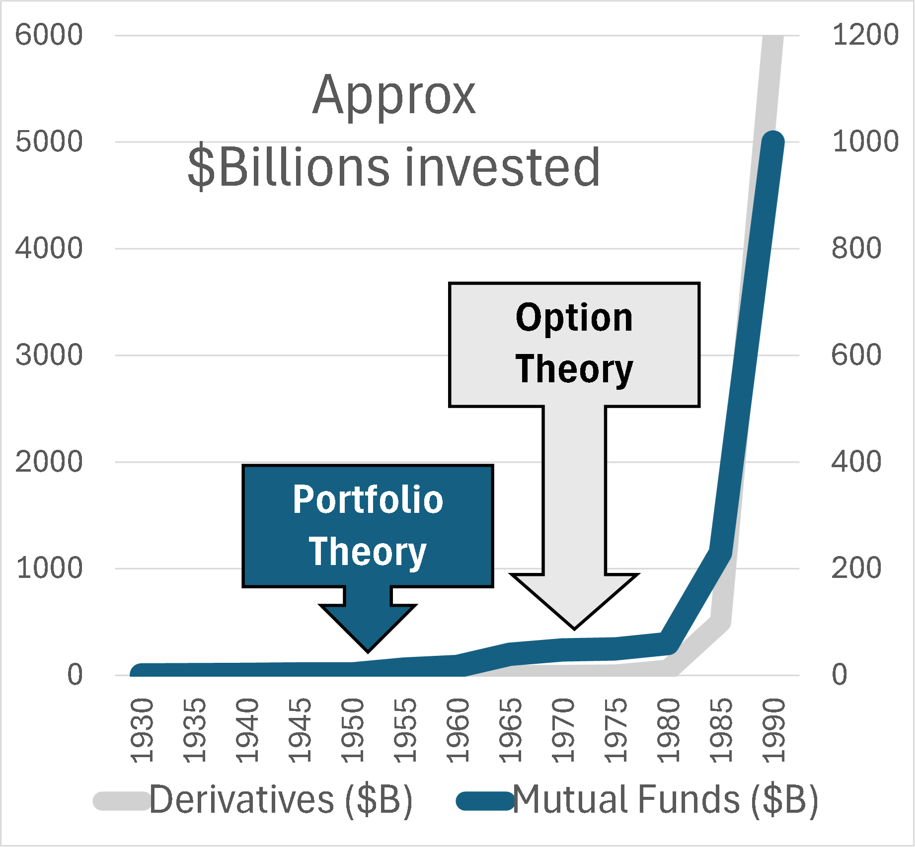
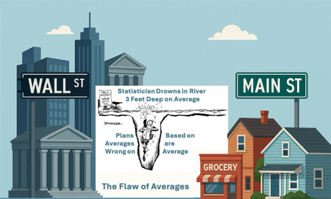
Decades later when I wrote a book on the subject, I called it the Flaw of Averages, not Jensen’s Inequality because I didn’t want to trigger PTSD*. Most managers are still unaware of this general principle, even though it must cost the economy plenty in unnecessary costs and missed opportunities. A notable exception is the $trillion derivatives market that emerged after the Black Scholes equation successfully related the average value of an option to the uncertain value of the underlying asset.
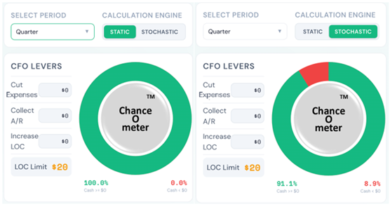
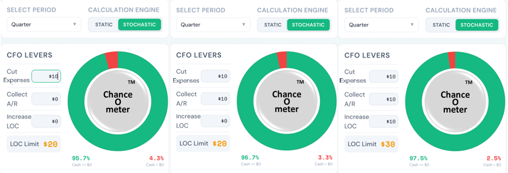
In general, it has just been too complicated to take uncertainty into account without creating elaborate simulations that weren’t flexible enough for on-the-spot decisions. All that has changed with Stochastic Data and AI, as described in a June 2026 article in ORMS Today.
So, the time has come to rub people’s noses … er I mean explain Jensen’s Inequality yet again. My neighbor, Pooja Bucklin, a math major herself makes a compelling pitch in three 1 minute videos below.
* Post Traumatic Statistics Disorder
Copyright © 2026 Sam L. Savage