The Only Valid Excuse for not Quantifying Uncertainty

by Sam L. Savage

“It is difficult to get a man to understand something, when his salary depends on his not understanding it”
— Upton Sinclair

According to my new best friend and advisor, ChatGPT, the above quote from the 1906 book, “The Jungle,”

“reflects Sinclair's belief that the interests of capitalists often conflict with the well-being of workers and the general public, and that people will often choose to ignore or justify harmful practices if they stand to benefit financially from them.”

Although the context of the quote was

“the unsanitary and inhumane conditions in the meatpacking plants and the corrupt practices of the industry, such as the manipulation and adulteration of food products,”

it applies equally well today to

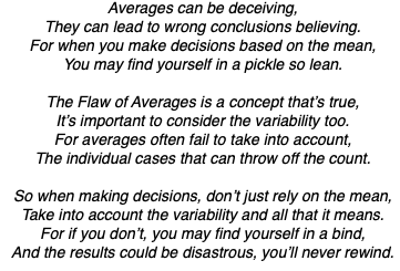
The unsound and inaccurate computations in the realm of uncertainty and the common practices in industry to use averages that introduce systematic errors, in short, the Flaw of Averages.

With a few notable exceptions business is conducted with single number estimates that pass between analysts (who know better), information systems and decision makers. Until now, you couldn’t just quantify uncertainty at one of these nodes and have it propagate through the organization. Those insisting on probabilistic representations were misfits, who might ultimately lose their salary. So many people know that this is wrong, however, that it has become necessary to ignore or justify these harmful practices.

Doug Hubbard is author of the How to Measure Anything series, the Failure of Risk Management, and other important books on quantifying uncertainty. As brothers in arms in the War on Averages, we have shared numerous examples of clients who are strongly motivated to not understand uncertainty. This has resulted in

The Savage and Hubbard Top Ten List

of Lame Excuses for Not Quantifying Uncertainty

But Sinclair’s quote reminds us that it is not just intellectual laziness and post traumatic statistics disorder (PTSD) holding people back, but also job security.

Financial Engineering and Physics

Financial engineering was a great victory in the War on Averages. In 1973, Fischer Black and Myron Scholes published The Pricing of Options and Corporate Liabilities.” It contained the famous Black-Scholes equation for pricing options that solved a specific case of the Flaw of Averages. It showed that valid option pricing requires the probability distribution of the future asset price, not just the average. They relied on the work of physicist, Albert Einstein, on the Brownian motion of gas particles. It led to the $Trillion Derivatives industry and eventually a Nobel Prize. Although the Black-Scholes formula was not perfect it was vastly better than the alternatives, and those who chose to ignore or justify the harmful practices of using averages were the ones who lost their salaries, often to be replaced by physicists.

Chancification

My recent book on Chancification shows how today, the revolutionary quantification of uncertainty that began in finance can spread to many other sectors without anyone losing their salaries. But how?

Analysts are by and large already quantifying uncertainty but can’t convey it as such in corporate databases, nor would decision makers know what to do with it if they got it. ProbabilityManagement.org has now developed tools and standards to transition organizations into the Chance Age by integrating existing decision-makers, analysts, and IT systems, without requiring any new hires or significant software development. But how?

The secret sauce, no make that the open-source sauce, is the SIPmath™ 3.0 Standard, which can convey millions of simulation trials in as little as a few hundred bytes of JSON data, based on the HDR pseudo random number generator of Doug Hubbard, and the remarkable Metalog Distribution of Tom Keelin. JSON (JavaScript Object Notation) is a common data-interchange format that can be interpreted by humans and machines. It is easy to generate SIPmath 3.0 JSON files from nearly any form of analytics. But how?

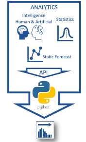
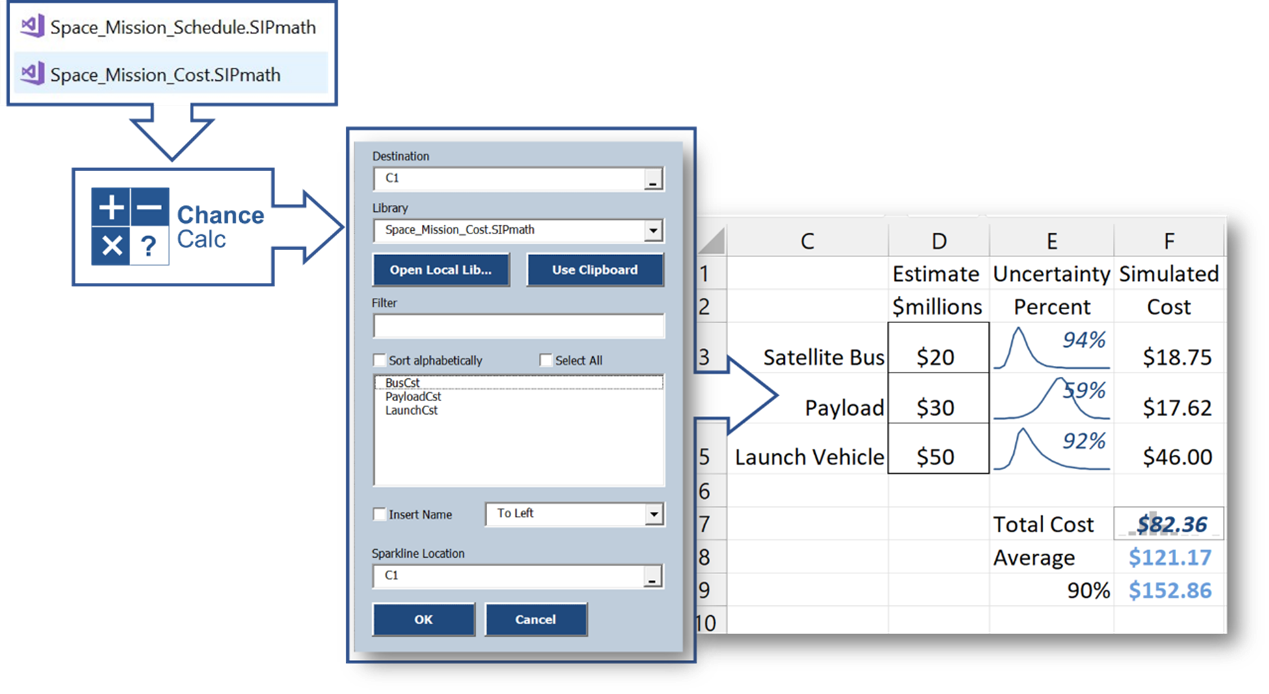
Open-source Python code reads standard analytics output through an API (Application Programming Interface) recently developed by the nonprofit. The files produced may be interpreted by virtually any software platform, including native Excel so managers can start making Chance-Informed decisions. But how?

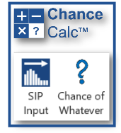
The ChanceCalc Excel add-in, developed by ProbabilityManagement.org, requires a manager to learn only two new commands: Input SIP and Chance of Whatever as shown in the video below.

Give Chance a Chance

Do you want to learn more? Join me for one of my webinars and receive a free copy of ChanceCalc ($150 value). To register, visit Welcome to the Chance Age Webinars.

© Copyright 2023, Sam L. Savage

ChatGPT Waxes Poetic on the Flaw of Averages and Metalog Distribution

When I was a PhD student in computer science, I remember opening a book on recursive function theory. In the introduction it stated that a mathematical equation that I found inscrutable was obvious. I thought: “This book ain’t for me,” and I put it down, never to pick it back up. But the statement nagged at me and a few days later, in a thunderclap of insight, I proved the equation to myself, and my mind was off to the races. For a couple of days and nights, including in my dreams, I searched for parallel mathematical examples, and simultaneously learned something about my own thought processes.

A creative part of my mind would proudly walk into my head with some random idea and say: “Is this an example of the equation?” Then 95% of the time, a judgmental side of my brain would say: “That’s total BS!” But occasionally, the judge would say: “You might have a point there.” What struck me at the time was how totally random the creative part was. Once, when I was asleep, it absurdly suggested that an example of the equation was an element of a weird, irrelevant dream! The judge kicked me out of the courtroom for that one and I woke up.

There is no doubt that random association plays a key role in creativity, and  Mozart and other musicians of the time created random algorithms for composing music. Perhaps this was a distant ancestor of ChatGBT, which is described in Wikipedia as of 12-28-2022 as follows:

ChatGPT (Generative Pre-trained Transformer is a chatbot launched by OpenAI in November 2022. It is built on top of OpenAI's GPT-3.5 family of large language models and is fine-tuned with both supervised and reinforcement learning techniques.

ChatGPT certainly has its random association down. Here is what it produced within ten seconds of being asked to write a poem on the Flaw of Averages.

Of course, you know I would never settle for a single point estimate. My colleague, Matthew Raphaelson tried it on his machine, and on his first attempt got something quite similar. Perhaps it always starts with the same random number seed. But on his second request he got the following:

Now how about ChatGPT’s judgement? It’s not great. In a few experiments it got factual stuff quite wrong. But so, what. Imagine ChatGPT playing the role of the crazy random thought generator, and a human paying the role of the judge.

I tried this with a poem on the Metalog Distribution as follows:

“Write a Poem on Metalog How I love Thee let me count the ways. This is about the Metalog Probability Distribution.”

It started out with:

Stop the presses! The whole point of the Metalog is to go beyond the bell curve.

So, I provided more guidance as follows:

“Write a Poem on Metalog How I love Thee let me count the ways. This is about the Metalog Probability Distribution which can mimic other distributions both symmetric and asymmetric.”

And it came up with:

Sheesh! (quoting the Metalog’s inventor, Tom Keelin, when he saw this).

I would not have received D’s in three out of four years of high school English if I had had ChatGPT. And let’s not forget that the human brain, even with medical breakthroughs, can only grow smarter for as much as 100 years. How long will ChatGPT and its ancestors grow smarter? Forever!

© Sam L. Savage, 2023

Merry Chancemas


2022 Ushered in the Chance Age

Here's what is coming in 2023 

  • A summit on Chancealytics in Pittsburgh in May

  • A Chancification bootcamp

  • Chancipedia

  • The ChanceOmeter

Chance Awareness is minimal today or I wouldn’t have been able to purchase the .com domains for ChanceAge, Chancification, ChanceInformed, ChanceTalk, ChanceCalc, Chancealytics, Chancipedia, ChanceOmeter, ChanceAware and ChanceAwareness for $11.99 each. We will make the world more Chance Aware in 2023. Oh, I almost forgot. As a shopaholic I couldn’t resist picking up Chancemas.com today.

Happy New Year from

ProbabilityManagement.org

Join the Chance Age with Our Latest Tools

by Sam L. Savage

“We shape our tools and thereafter our tools shape us”

— John Culkin

I knew my world had changed in August of 2012 when I discovered that the Data Table function in Excel had become powerful enough to perform practical Monte Carlo simulation without any add-ins. This inspired me to shape an evolving family of tools for creating standalone Excel simulations. These, in turn, have shaped me back in more ways than I can count, in my teaching and consulting practice. Eventually I converged on two buttons that ushered in the Chance Age: SIP Input, and Chance of Whatever.

Our latest tools provide up to three ribbons.

The ChanceCalc ribbon is for making chance-informed decisions based on SIP Libraries created in other programs. Notably, ChanceCalc can read the latest SIPmath™ 3.0 Standard generated by Frontline System’s Analytica Solver. But it can also read SIPmath 2.0 libraries created with ChanceCalc Monte Carlo, Analytica from Lumina Decision Systems, and CSV files generated from @RISK and Crystal Ball.

The new Metalog ribbon copies Tom Keelin’s Metalog Distributions out of his elegant Excel templates and provides several options for pasting or linking them into your model or saving them as SIPmath 3.0 JSON libraries. 

Finally, ChanceCalc Monte Carlo adds a third ribbon that rolls in all the power of our legacy Enterprise SIPmath Tools, with additional important Import and Export features.

And remember, that all the tools in the SIPmath family perform interactive simulation in native Excel through the Data Table so the models created with the tools do not require the tools to run.

The Marketing Funnel Fallacy

by Dr. Sam L. Savage

The Funnel

My colleagues Bridget Cash, Matthew Raphaelson, and I have recently been examining Chance-Informed marketing decisions. It is common to view the transition of a potential customer from first awareness of a product to purchase as a funnel. As a simplified example, consider an email list of 5,000,000 potential customers. Suppose you believe that 10% of these will visit your site. Of those that do, 50% will move on to your Products page, and 40% of those will move on the shopping cart and make the purchase.

But Are You Certain?

Typically, these probabilities are not known with certainty. They may be estimated with Beta distributions or other methods. Let’s assume that the percentages are the correct average of the funnel probabilities, but that they are uncertain with independent errors as shown. Then the funnel fallacy can be stated as follows.

The Fallacy

On Average the Conversion Rate will be the Product of the Probabilities

BUT

The Chance is Over 50% that the Conversion Rate will be Below Average 

Why? When you multiply positive uncertainties together, they skew to the left. The most famous example of this is the normal distribution, which comes from adding independent variables together to make a symmetric distribution and the lognormal distribution which comes from multiplying independent variables together to make a skewed distribution. But skewed to the left implies that more of the distribution is to the left of the average than to the right.

This means that when you are estimating conversion rates based on average funnel probabilities, you will get the correct average, but (and this is the legal term of art) More Likely Than Not you won’t achieve your target. And because this is a universal mathematical fact, you (and here is another legal term of art) Know This or Should Know This.

If you are involved in marketing, hiring, product development, or any other funnel driven enterprise, keep the above in mind the next time you are setting expectations.

I will be discussing the Marketing Funnel Fallacy in my Welcome to the Chance Age webinar series, taking place on September 28 and 29. I hope to see you there.

© Copyright 2022, Sam L. Savage

Chancification in Cost Estimation

by Sam L. Savage

In my blog post Making Your S Curves Actionable,” I described my introduction to ICEAA, the International Cost Estimating & Analysis Association. Christina Snyder, Vice President of the ICEAA, and Patrick Malone of Systems Planning and Analysis Inc., an ICEAA member, have assisted me in developing cost estimation examples for future versions of my Welcome to the Chance Age webinar series. We have recently added webinars on September 28 and 29.

ICEAA members already make probabilistic cost estimates based on standalone simulations using such packages as @RISK and Crystal Ball, so they are already halfway to Chancification. What would it take to get them all the way, and so what if they did?

What Would It Take?

Very little. As a reminder, Chancification conveys arrays of simulation trials (SIPs or Stochastic Information Packets) between applications much as electrification conveys electricity between power plants and end users. The simplest way to do this is with the cockroach of all data formats, the CSV file, which can be easily generated from virtually any simulation system. But just as in electrification there is both direct and alternating current of various voltages, in Chancification there are more structured formats, including the open SIPmath™ 3.0 Standard that can generate up to 100 million random variates of almost any distribution along with metadata in a very small JSON file.

So What?

Here are several benefits of Chancification:

  1. Large simulations may be aggregated from small simulations. Imagine a simulation of operating expense for a single aircraft, which takes the cost of fuel into account. To simulate a fleet of 100 such aircraft, today one might just add 99 planes to the simulation you already had. But sooner or later such models collapse under their own weight. Chancification provides an alternative. Each of the 100 aircraft can be simulated separately in various computational platforms. The only requirement is that they use the same SIP of fuel price (and any other global inputs). That way the output SIP of each plane is coherent with the other SIPs in the fleet, as they use precisely the same fuel price on each trial. This in turn means they may be added together to create the SIP of fleetwide cost.

  2. Once the SIP Libraries are generated by the data scientists and statisticians, they may be used in chance-informed decisions by non-statisticians in any environment, including native Excel.

  3. If the 18th century economist Adam Smith was correct, we may see specialization within the industry, with some firms focused on selling high fidelity stochastic libraries of the costs of components, while others focus on assembling these libraries into models of large systems. This will only be possible with standard data formats for moving SIPs from producers to consumers.

I hope you can join us at my Welcome to the Chance Age webinar series to learn more about Chancification in cost estimation and many other areas.

100 Million Monte Carlo Trials in 88 Bytes!

ProbabilityManagement.org Announces the Metalog Interface

by Sam L. Savage

Wait a Minute!

Claude Shannon’s information theory says you can’t store 100 million numbers in 88 bytes.

True, but Tom Keelin’s Metalog distribution, driven by Doug Hubbard’s HDR pseudo-random number generator, can create identical streams of up to 100 million random variates on any platform. Now ChanceCalc 1.3, currently in beta, includes an interface to Tom Keelin’s elegant Excel Metalog templates. Using these templates, you can create 3.0 JSON libraries or paste Metalog simulation formulas directly into Excel for use with ChanceCalc, the SIPmath Modeler Tools, @RISK, or Crystal Ball

How Does This Work?

Like Taylor series, Metalogs can take any number of terms (see Wikipedia). But for practical purposes, 18 parameters will model virtually any continuous distribution you will face. In its standard configuration, the HDR generator takes up to four initialization seeds, which provides great flexibility when sharing SIPMath™ 3.0 Libraries with others. The version of the HDR built into our tools, which has been limited in numerical accuracy to support Excel, can generate 100 million random numbers before the rubber band breaks (or rather, before the results on the dieharder test deteriorate). So that’s a total of 22 input parameters (88 bytes) to generate nearly any distribution. The open SIPmath 3.0 Standard wraps these 22 parameters in JSON objects containing metadata that can be used in Excel, Python, R, or virtually any other computer platform.

The first commercial package to read and write the SIPmath 3.0 Standard was Frontline Systems’ Analytic Solver. This powerful Excel add-in performs both simulation and optimization, including stochastic optimization. Our new interface lets you use Tom’s templates directly.

Want to Learn More?

We are looking for beta testers for this new software. All those interested in becoming beta testers will need to attend a free information session where I will demonstrate the software.

Watch Sam Savage and Alex Sidorenko discuss the new Metalog interface

© Copyright 2022, Sam L. Savage

The SIPply Chain Forum

by Sam L. Savage

The man who knows HOW will always have a job.
The man who also knows WHY will always be his boss.

— Ralph Waldo Emerson

I have now delivered my first few Welcome to the Chance Age webinars, and they have inspired a new initiative, the SIPply Chain Forum. I will lead a series of monthly web gatherings in which I and my fellow combatants in the War on Averages will share their experiences in developing SIP libraries. This will start out as an invitation-only event, open to attendees of the webinar series, who are invited at no expense to join me for the latest developments and present their own work. Attendees from the first sessions are grappling with uncertainties ranging from public housing revenues to the sales of building supplies to the impact of cyber-attack.

As a reminder, SIPs are standardized data structures for conveying uncertainty, developed and promulgated by ProbabilityManagement.org. Once uncertainties such as those described above are translated into SIPs using the SIPmath™ Standard format, any Excel user with the ChanceCalc add-in can easily use them to illuminate the chances of meeting specified goals. But where do SIPs come from? Ideally from statistical experts and data scientists, for use by decision makers without such skills. This is analogous to electrical engineers producing the power to illuminate the lightbulbs of non-engineers.  

But if probability were electricity, it would be 1895, the date of Westinghouse’s first hydro powerplant at Niagara Falls, so we should all consider ourselves pioneers. The reason WHY we fight averages is because they result in dumb outcomes known collectively as the Flaw of Averages. However, many of you don’t know HOW to create SIP Libraries. But this is what Statisticians and data scientists do know HOW to do, so according to Emerson, they will eventually be working for us.

In the meantime, in the SIPply Chain Forum, we will collaboratively build small prototype libraries and study a growing body of examples, ranging from the Covid Hospitalization Library generator developed by Eng-wee Yeo of Kaiser Permanente to the portfolios of petroleum exploration projects at Shell that kicked off the discipline of probability management. 

At this point ChanceCalc can read three different file formats, which may be produced by a wide range of software packages. I have summarized these in the table below. I look forward to seeing you at one of our SIPply Chain Forums where we will all be learning how to move into the Chance Age together.

Making Your S Curves Actionable

Illustration of the "Ugly Duckling" by Milo Winter, a renowned illustrator (August 7, 1888 – August 15, 1956), first published in 1916 in the United States in the book "Hans Andersen's Fairy Tales."

Finding My Flock

by Sam L. Savage

I typically don’t pick up a lot of friends by discussing probability in polite company, leaving me feeling like the ugly duckling in the fairy tale. But earlier this month I attended a meeting of the International Cost Estimating & Analysis Association (ICEAA), at which I felt like I finally found my flock of swans.

This nonprofit organization is devoted to improving cost estimation in the face of uncertainty as required by the Department of Defense Estimating Guide. By definition, they are all applied statisticians. The talks I attended were practical but rigorous, on subjects as diverse as reducing the expense of space launch vehicles, assessing the costs of climate change, and pooling resources to create a new generation of small nuclear reactors. Unlike some meetings I have attended, the audience did not bolt for the door as soon as the session ended but stuck around to ask questions. It was very refreshing.

Everyone in this group is familiar with probability distributions. They generally view these as S Curves, since it is easy to read probabilities directly off them. But when they need to perform calculations with distributions, they typically revert to Monte Carlo simulation. Most were unaware that with probability management, you can sum uncertainties directly as data (or perform any other calculation for that matter).

My keynote presentation was entitled Making S Curves Actionable, and it described a proof of concept I developed with Christina Snyder, an experienced cost analyst and Vice President of the ICEAA. Suppose you had an S Curve for the development of a new missile system, and another S Curve for the per unit manufacturing cost of the missiles. Then to find the total program cost for 150 of the missiles, the current approach would be to run a Monte Carlo simulation based on the two S Curves. Christina and I created a 3.0 SIPmath library in JSON that allowed us to calculate Program Cost as S Curve1 +150 x S Curve2 using ChanceCalc.

I am excited by the potential synergy between the two nonprofits and hope to continue working with Christina and others at ICEAA to combine our open standards and technologies with their best practices in costs estimating. Stay tuned for more soon.

In the meantime, we have added more dates in July and August for my highly interactive Welcome to the Chance Age webinar series. As a reminder, attendees receive a free copy of ChanceCalc, a free Kindle copy of Chancification: How to Fix the Flaw of Averages (valid only for U.S.-based email addresses), and $200 off the Enterprise SIPmath Tools.


Introducing the First Online Generator in the Probability Power Grid

by Sam L. Savage

Here is an exciting new online application to generate ChanceCalc-compatible SIPmath 3.0 JSON libraries. As input, it can take either a CSV file of Monte Carlo trials, or a list of Quantile value estimates of an expert.

This app will be made available to attendees of my “Welcome to the Chance Age” webinars, where I will explain its use.  

CSV Mode

In this mode, the app takes in CSV files generated from any Monte Carlo package such as @RISK or Crystal Ball. The user has the option to have the app calculate correlation coefficients between variables, or model them as independent.

Quantile Mode

This mode is perfect for capturing expert opinion. In this mode, if correlation is desired, the user must enter the coefficients.

Welcome to the Chance Age!

There are lots of ways to get involved: