The Copula Layer of the 3.0 Standard
The Copula Layer imposes interrelationships between variables in the SIPmath 3.0 Standard as described in the four sections below.
CSV Files and the SIPmath 2.0 Standard
The 3.0 Standard
Copulas
Factor Models
CSV Files and the SIPmath 2.0 Standard
With CSV files or the SIPmath 2.0 Standard, vectors of simulation trials (SIPs) are stored in a Stochastic Library Unit with Relationships Preserved (SLURP) and no Copula Layer is needed. That is, any statistical interrelationships are baked into the data during simulations. The disadvantages are that the sizes of the files can grow very large, and that the number of trials may not be changed.
The 3.0 Standard
The SIPmath 3.0 Standard is based on driving the Inverse Cumulative function of a variate with a Uniform 0,1 random number, which may be viewed as the result of a game-board spinner going between 0 and 1. An example of this approach in Native Excel is NORM.INV(RAND(),MEAN,STDEV), where RAND() is the built in Uniform 0,1. In the SIPmath 3.0 Standard, RAND() is replaced by a cross-platform seed-able Pseudo Random Number Generator (PRNG), for which currently the HDR 2 is supported. Instead of NORM.INV, which represents only a single distribution, the standard currently supports Metalog 1.0 and 2.0 parameter driven Quantile (F-Inverse) functions, which closely approximate a wide array of continuous distributions. With this approach, each software platform only needs to support a few functions instead of hundreds of separate Quantile functions. For discrete random variants, Probability Tables are used instead of Quantile functions. The parameters for all functions and tables are stored with Metadata in small JSON data files.
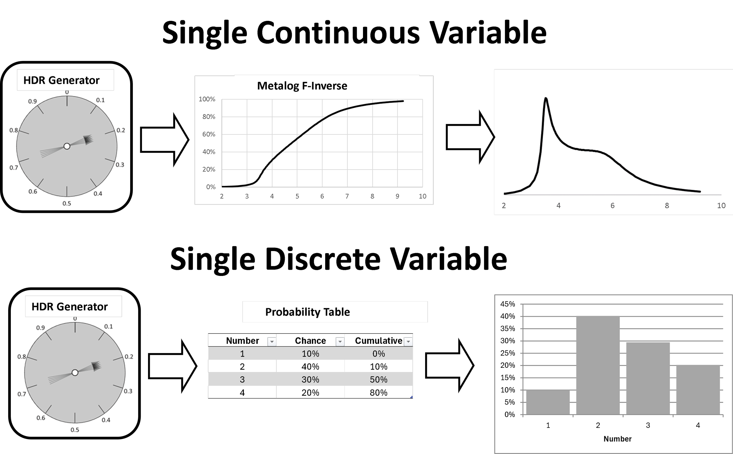
The resulting storage requirements can be several orders of magnitude smaller than those of the SIPmath 2.0 generated data, and furthermore the number of trials may be changed, with an upper limit exceeding tens of millions. The disadvantage is that PRNG and Quantile Functions alone do not impose statistical interrelationships between generated random output variables. This may be accomplished through either a Copula or a Factors Model.
Copulas
In statistics a copula imposes an interrelationship between statistical variables without changing the shapes of their distributions [i]. This is the function of the Copula Layer in the SIPmath 3.0 Standard. It does this by imposing the desired interrelationships on the relative rankings of the Uniform 0,1 random numbers, which then pass them on to either the Quantile Functions or Probability Tables.
Two classes of Copula are supported, Computational and Empirical:
Computational Copulas
Computational Copulas impose statistical interrelationships on independent Uniform 0,1 variables by blending them together in various ways. The resulting dependent Uniform 0,1s form the Copula Layer, and drive the F -Inverses to create dependent output variables. Examples include, Gaussian and Vine Copulas.
Empirical Copulas
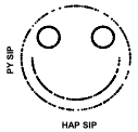
With Empirical Copulas the Copula Layer consists of SIPs of Uniform 0,1s in specified rank orders that impose the same set of rank orderings on the output variables. The rank orderings can be virtually anything. Consider for example, a scatter plot of 1,000 points creating a Happy Face. The SIP of 1,000 X points is defined as HAP, and the SIP of corresponding Y points as PY. An Empirical Copula based on relative rankings of HAP and PY will be demonstrated with an illustrious Metalog distribution.

Dr. Tom Keelin, inventor of the Metalog, is also an avid catch-and-release fly fisherman, shown here with a huge steelhead trout. Having access to the recorded weights of over three thousand steelhead, he naturally wondered about the distribution and fit a Metalog.
To his surprise, he discovered that it was bimodal [ii]. This might make one question whether the Metalog had overfit the data.
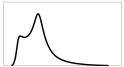
Biologists confirmed that this made perfect sense. Steelhead belong to the same genus as salmon, with both fattening up in the ocean, and then swimming upstream to spawn in fresh water but there is a big difference. Salmon inevitably die after copulation (same root as copula), while steelhead swim back down to the ocean for another meal or two. The two modes denote what are known as “1-salt” fish on the lighter end, and “2-salt” fish at the heavier. Perhaps there are 3, 4 and higher in the data but only two modes are visible.
So, what would happen if two steelhead distributions were joined by an empirical happy face copula?
Here are the steps:
Replace the HAP SIP and PY SIP with Uniform 0,1 SIPs with the same rank orders as HAP and PY. This is simply a matter of sorting one Uniform according to HAP to create HAP Rank and one according to PY to create PY Rank.
Drive the steelhead Metalog with HAP Rank to get Steelhead 1 and with PY Rank to get Steelhead 2.
Create a scatterplot of Steelhead 1 and Steelhead 2, and voila, a Happy Fish!
Factor Models
Factor models explain interrelated uncertainties by decomposing outcomes into a small number of common or global factors plus idiosyncratic or local uncertainties. The canonical example is William F. Sharpe’s Capital Asset Pricing Model (CAPM) [iii] which represents asset returns as exposure to a single systematic market factor, such as the S&P 500, and the individual independent volatility of each asset, which ultimately may be diversified away. The foundational 2005 article in OR/MS Today [iv] on Probability Management extends this same idea beyond finance to portfolios of petroleum exploration projects for Royal Dutch Shell. Here the local uncertainties were the outcomes at any particular project, while the global factors involved prices and geopolitics, which impacted all projects at once. This may be accomplished with a single SIP Library for global factors and a separate library for each project, with the interrelationships imposed by the direct dependency of the projects on the external factors.
[i] https://en.wikipedia.org/wiki/Copula_(statistics)
[ii] Thomas W. Keelin (2016) The Metalog Distributions. Decision Analysis 13(4):243-277.
[iii] William F. Sharpe (1964).
Capital Asset Prices: A Theory of Market Equilibrium under Conditions of Risk.
Journal of Finance, Vol. 19, No. 3, pp. 425–442.
[iv] https://www.probabilitymanagement.org/s/Probability_Management_Part1s.pdf